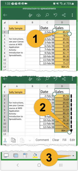
- Tap the cell you want to format to currency. Or tap the first cell in a range of cells that you want to format to currency. This will create a box around the cell with a circle at the bottom.
- Tap, hold, and drag the circle so the box surrounds all the cells you want to format to currency. In this case, we surround cells D2 to D12.
- Tap the main menu icon, which looks like a small arrow in the bottom right corner.

- The main menu contains many other menus. Make sure you are on the submenu called "Home."
- Scroll down the Home menu options and tap the arrow next on the "Number Format menu item."
- On the Number Format menu, tap "Currency." This will format the cells you selected to currency using the default symbol.
- To choose the symbol, tap the arrow on the "Currency" menu item.
- Scroll down and tap the arrow on the "More Symbols" menu item.

- In this case, we are selecting "$ English (United States)."
- Doing so ensures that the $ symbol is used in the selected cells (cell range).

Important! Ensure that you also format cells K2 to K7 and cells N2 to N7 for correct dollar symbols. Follow the same steps as performed for cells D2 to D12.