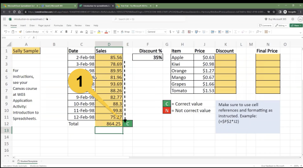
1. Click on the cell you want to format to currency. Or click on the first cell in a range of cells that you want to format to currency. This will create a box around the cell with a square at the bottom.
2. Click, hold, and drag the square so the box surrounds all the cells you want to format to currency. In this case, we surround cells D2 to D12.

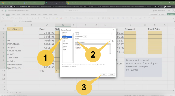
1. Right-click on the highlighted cells to reveal a menu. On the menu, click "Number Format."

1. Click "Currency."
2. Make sure that you have selected the $ symbol.
3. Click "Ok".

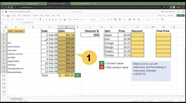
1. The selected cells are now formatted for currency using the $ symbol.

Important! Ensure that you also format cells K2 to K7 and cells N2 to N7 for correct dollar symbols. Follow the same steps as performed for cells D2 to D12.